🕯️ GPT2-finetuning internal constructs
1.1 tokenizer
The processing part of the dataset is inside encode.py:
def main():
   args = parser.parse_args()
   enc = encoder.get_encoder(args.model_name, models_dir=args.models_dir)
   print('Reading files')
   chunks = load_dataset(enc, args.in_text, args.combine, encoding=args.encoding)
   print('Writing', args.out_npz)
   np.savez_compressed(args.out_npz, *chunks)
Most NLP pre-trained models use embeddings to represent word meanings. In gpt, byte pair encoding (BPE) method is used for word segmentation.
Here is how the bpe inside encoder.py is implemented in gpt2-finetuning
# Representing words as unicode codes
def bytes_to_unicode():
    """
    Returns list of utf-8 byte and a corresponding list of unicode strings.
    The reversible bpe codes work on unicode strings.
    This means you need a large # of unicode characters in your vocab if you want to avoid UNKs.
    When you're at something like a 10B token dataset you end up needing around 5K for decent coverage.
    This is a signficant percentage of your normal, say, 32K bpe vocab.
    To avoid that, we want lookup tables between utf-8 bytes and unicode strings.
    And avoids mapping to whitespace/control characters the bpe code barfs on.
    """
    bs = list(range(ord("!"), ord("~")+1))+list(range(ord("¡"), ord("¬")+1))+list(range(ord("®"), ord("ÿ")+1))
    cs = bs[:]
    n = 0
    for b in range(2**8):
        if b not in bs:
            bs.append(b)
            cs.append(2**8+n)
            n += 1
    cs = [chr(n) for n in cs]
    return dict(zip(bs, cs))
#bpe breaks down each word
# e.g. Decompose (" hello") into ("h""e","e""l",""l"l"...)
def get_pairs(word):
    """Return set of symbol pairs in a word.

    Word is represented as tuple of symbols (symbols being variable-length strings).
    """
    pairs = set()
    prev_char = word[0]
    for char in word[1:]:
        pairs.add((prev_char, char))
        prev_char = char
    return pairs
# The encoder is called before training starts
class Encoder:
    def __init__(self, encoder, bpe_merges, errors='replace'):
        self.encoder = encoder
        self.decoder = {v:k for k,v in self.encoder.items()}
        self.errors = errors # how to handle errors in decoding
        self.byte_encoder = bytes_to_unicode()
        self.byte_decoder = {v:k for k, v in self.byte_encoder.items()}
        self.bpe_ranks = dict(zip(bpe_merges, range(len(bpe_merges))))  #bpe_merges is represented as the common rank of each term
        self.cache = {}

        # Should haved added re.IGNORECASE so BPE merges can happen for capitalized versions of contractions
        self.pat = re.compile(r"""'s|'t|'re|'ve|'m|'ll|'d| ?\p{L}+| ?\p{N}+| ?[^\s\p{L}\p{N}]+|\s+(?!\S)|\s+""")#Some operations on special characters will be used later
#If the word is in the internal cache, it is returned
def bpe(self, token):
       if token in self.cache:
           return self.cache[token]
       word = tuple(token)
       #Perform the getpairs operation
       pairs = get_pairs(word)
       #If the pair is not separate, the full word is returned, but if the word is very short
       if not pairs:
         return token
       #Operate on pair word pairs
       while True:
          # Sort the input pairs according to the.bpe file (commonly used ranking). Here the pair is the 55 line mentions a, b
          # Find the most common pair float('inf') means infinity If you can't find it return infinity to avoid being selected
          bigram = min(pairs, key = lambda pair:
          #By what sort is the key equivalent in MIN MAX
          self.bpe_ranks.get(pair, float('inf')))
           # The combination is not in the bpe table pairs can no longer be split End of loop
           if bigram not in self.bpe_ranks:
               break
            # Get the first word and the second word
           first, second = bigram
           new_word = []
           i = 0
            #  Finding a substring
           while i < len(word):
               try:
                   j = word.index(first, i)# i means search from the ith # find list.index(x, start position, end position) # find the first word in the passed word What this means is that since the pair is unordered we need to find the order of the input words
                   new_word.extend(word[i:j])# Place the substring first=word[i:j] in the new_word variable
                   i = j
               except:
                   new_word.extend(word[i:])#The i: slice is directly put in when J is out of bounds
                   break
               #This means that if the first and second are connected they will be added to new_word as a whole
               if word[i] == first and i < len(word)-1 and word[i+1] == second:
                   new_word.append(first+second)
                   i += 2
               else:
                   new_word.append(word[i])
                   i += 1
           #Recursive operations
           new_word = tuple(new_word)
           word = new_word
           if len(word) == 1:
               break
           else:
               pairs = get_pairs(word)
       word = ' '.join(word)
       #Put the word in the cache
       self.cache[token] = word
       return word
# The word encoding process that is not in the self.encoder dictionary
def encode(self, text):
    bpe_tokens = []
    #Self.pat.findall text means take the pattern of self.pat from the text and that means she's becomes she s
    for token in re.findall(self.pat, text):
        token = ''.join(self.byte_encoder[b] for b in token.encode('utf-8'))
        #This is roughly equivalent to token = unicode(token, "utf-8") # converting the text to utf-8 and using the dict produced by self.byte_encoder -- bytes_to_unicode() back into character form and concatenating it into a string
        bpe_tokens.extend(self.encoder[bpe_token] for bpe_token in self.bpe(token).split(' '))
         #This list is returned by looking up the split words in the passed embedding dictionary
    return bpe_tokens
This is encoder.py. encoder.py is a method for bpe words in encode. Now return the line in encode.py
python
chunks = load_dataset(enc, args.in_text, args.combine, encoding=args.encoding)```
Here we apply the load_dataset.py function,
def load_dataset(enc, path, combine, encoding=None):
    paths = []
    if os.path.isfile(path):
        # Simple file
        paths.append(path)
    elif os.path.isdir(path):
        # Directory
        for (dirpath, _, fnames) in os.walk(path):
            for fname in fnames:
                paths.append(os.path.join(dirpath, fname))
    else:
        # Assume glob
        paths = glob.glob(path)

    token_chunks = []
    raw_text = ''
    for path in tqdm.tqdm(paths):
        if path.endswith('.npz'):
            # Pre-encoded
            with np.load(path) as npz:
                for item in npz.files:
                    token_chunks.append(npz[item])
        else:
            # Plain text
            with open(path, 'r', encoding=encoding) as fp:
                raw_text += fp.read()
            if len(raw_text) >= combine:
                tokens = np.stack(enc.encode(raw_text))
                token_chunks.append(tokens)
                raw_text = ''
            else:
                raw_text += '<|endoftext|>'
    if raw_text:
        tokens = np.stack(enc.encode(raw_text))
        token_chunks.append(tokens)
    return token_chunks
1.2 model function
First, the body of the model The model function is as follows:
#Input for X and past:

#X is the language model input and past is the state that generated the above.
# When training, X is a set of training data [2] and past is empty.
# Conditional generation initial phase, X is a conditional statement, past is empty
# unconditionally generate initial phase, X is [end], past is empty
# In generation, X is the last generated word, and past is all previous K's and V's.
def model(hparams, X, past=None, scope='model', reuse=tf.AUTO_REUSE):
    with tf.variable_scope(scope, reuse=reuse):
        results = {}
        batch, sequence = shape_list(X)

        wpe = tf.get_variable('wpe', [hparams.n_ctx, hparams.n_embd],
                             initializer=tf.random_normal_initializer(stddev=0.01))
        wte = tf.get_variable('wte', [hparams.n_vocab, hparams.n_embd],
                             initializer=tf.random_normal_initializer(stddev=0.02)) #vte vpe word vector matrix wte word embedding matrix wpe position embedding matrix
        past_length = 0 if past is None else tf.shape(past)[-2]  #The length above has been generated
        h = tf.gather(wte, X) + tf.gather(wpe, positions_for(X, past_length))  #The information vte provided by the input x is summed with vpe. shape is [batch size, input length, embedding dimension]


        # Transformer
        presents = []
        pasts = tf.unstack(past, axis=1) if past is not None else [None] * hparams.n_layer
        assert len(pasts) == hparams.n_layer
        for layer, past in enumerate(pasts):
            h, present = block(h, 'h%d' % layer, past=past, hparams=hparams)   #h The final shape is [batch, seq, embd]
            if layer == 10:
                tf.add_to_collection('checkpoints', h)
            presents.append(present)
        results['present'] = tf.stack(presents, axis=1)
        h = norm(h, 'ln_f')            #Flattening h to [batch*seq,embd], multiplying the word embd transformation matrix by matrix multiplication (shape=[vocab,embd]), and finally reshape to get the final output logits

        # Language model loss.  Do tokens <n predict token n?
        h_flat = tf.reshape(h, [batch*sequence, hparams.n_embd])

        #
        logits = tf.matmul(h_flat, wte, transpose_b=True)
        logits = tf.reshape(logits, [batch, sequence, hparams.n_vocab])
        results['logits'] = logits
        return results
Let's start with part one
pythonresults = {} batch, sequence = shape_list(X) wpe = tf.get_variable('wpe', [hparams.n_ctx, >hparams.n_embd], >initializer=tf.random_normal_initializer(stddev=0.01)) wte = tf.get_variable('wte', [hparams.n_vocab, hparams.n_embd], initializer=tf.random_normal_initializer(stddev=0.02)) past_length = 0 if past is None else tf.shape(past)[-2] h = tf.gather(wte, X) + tf.gather(wpe, positions_for(X, past_length))
We first decompose each sentence into two weight matrices, wpe and wte, which are the word embedding vector and the word position encoding of the word.

 After processing the embedding, these matrices are sent up to the block,
python
presents = [] pasts = tf.unstack(past, axis=1) if past is not None else [None] * hparams.n_layer assert len(pasts) == hparams.n_layer for layer, past in enumerate(pasts): h, present = block(h, 'h%d' % layer, past=past, hparams=hparams)
if layer == 10: tf.add_to_collection('checkpoints', h) presents.append(present) results['present'] = tf.stack(presents, axis=1)
Now let's look at the blocks. Each block can be seen as a layer of data processing. It contains the self-attention mechanism, the feed-forward neural network, and the residual connection. 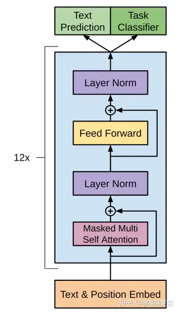
def block(x, scope, *, past, hparams):
    with tf.variable_scope(scope):
        nx = shape_list(x)[-1]
        a, present = attn(norm(x, 'ln_1'), 'attn', nx, past=past, hparams=hparams)  #Take the embedding dimension as nx and do Attention. Note that we are normalizing x before the Attention layer
        x = x + a   #The residual operation, where '+' is element-wise plus. x=a=[batch,seq,embedding], which adds up to [batch,seq,embedding].
        m = mlp(norm(x, 'ln_2'), 'mlp', nx*4, hparams=hparams)  #m is the feature further extracted by mlp.
        x = x + m #The information m residual obtained by mlp is added to the existing information x.
        return x, present     #Return the final result + present [batch, seq, embd]
The output of the previous layer is used as input in the block. Firstly, the residual of the known information x and the output a under the attention mechanism are added, where the self-attention operation is as follows:
- Create query,key,value vectors for each word
- For each input token, use its query vector to score the key vectors of all other tokens to obtain an attention score.
- Add the value vector by multiplying the attention scores from the previous step.
Where the q,k, and v vectors represent: query: is the representation of the current word used to score all other words (keys), we only need to focus on the query for the token we are currently working with.
Key: This can be thought of as a label for all the words in the sequence and is a reference when we are looking for related words.
Value: The actual representation of the word. Once we have scored the relevance of each word, we add the values to represent the value of the word we are currently processing.
1.2.1 Self-attention operations
Step 1: Create the query,key,value vectors  The equivalent operation in code is:
  c = conv1d(x, 'c_attn', n_state*3)
  q, k, v = map(split_heads, tf.split(c, 3, axis=2))
The convolution method is:
# This function linearly transforms x's nx features into nf features. It can be viewed as a 1D convolution or as a Linear layer.
#nx is the current number of features of x and start is the rest of the shapes. The shape_list function returns the shapes of x as a list.
#w is the parameter of linear in the first layer, defined as [1, the variable of the original feature number, the new feature number, and initialized with a normal distribution.
#b is the offset of the first layer linear, defined as a variable of the [new feature] number, and initialized with a constant value of 0.
#The statement #c is the result of a linear transformation is equivalent to C=WX+B
#The purpose of tf.reshape is to transform the result into the correct 3D shape. start+[nf] is the concatenation of the list, which, combined with the definition of start, converts nx to nf.
# reshape the inner layer into two dimensions, do matrix multiplication, add bias.
def conv1d(x, scope, nf, *, w_init_stdev=0.02):
    with tf.variable_scope(scope):
        *start, nx = shape_list(x)
        w = tf.get_variable('w', [1, nx, nf], initializer=tf.random_normal_initializer(stddev=w_init_stdev))
        b = tf.get_variable('b', [nf], initializer=tf.constant_initializer(0))
        c = tf.reshape(tf.matmul(tf.reshape(x, [-1, nx]), tf.reshape(w, [-1, nf]))+b, start+[nf])
        return c
Step 2: Calculate the attention score by dot multiplying the query of the first token with the key vectors of the other tokens via the query and key vectors to obtain the attention score of each token  Step 3: Sum, for each token, multiply the attention score obtained in the previous step with the value vector, and then accumulate the softmax to obtain the final attention score proportion
  The code for these two steps is contained in the multhead_attn method, which is explained shortly.
1.2.2 Self-attention with masks
The above is the self-attention mechanism in transformer. It should be noted that gpt uses self-attention with masked. It is different from ordinary self-attention in that for each token being processed, the attention score of the following token is 0, that is, only the input sentence before the current token will be focused
For example, in the input sequence "robot must obey orders". Each word is used as a token, and for the processing sequence batch size of 4, the model processes the entire sequence as a batch.  In this case, the token cannot directly calculate the attention score, so the query and key corresponding to the token need to be used to calculate the attention score
  After the multiplication is done, a mask matrix is added to mask out the words that are currently input.This is usually done by setting the mask matrix to an upper triangular matrix with very large negative values at the masked positions.
  Then softmax is applied to obtain the attention score:
  In the above table, it can be understood that when only one word robot is entered, the attention score of robot is 1, when the second word must is entered, the attention score of robot is 0.48, and the score of must is 0.52... You can see that each word is followed by a word attention score of 0
In the code, this is done in mask_attn_weights, which sets the weights matrix for the mask.
1.2.3 mask self attention in gpt2
Now suppose that the gpt2 model is used for prediction tasks, and the model adds a new word after each iteration. In order to increase the processing efficiency of the model, gpt2 does not simply multiply the attention of all previous tokens for each input token, but saves the previous token key and value vectors. Thus extracted in iterations 

 The qkv vector of the token in gpt2 is the concatenation vector of the query, key, and value of the token by multiplying the self-attention layer by the weight matrix.

 The value score of each head is obtained by splitting multiple heads.

The multi-head self-attention result is obtained by multiplying each value with its attention score. 

 Finally, the final result is obtained by merging multiple heads.
def attn(x, scope, n_state, *, past, hparams):
    assert x.shape.ndims == 3  # Should be [batch, sequence, features]
    assert n_state % hparams.n_head == 0
    if past is not None:
        assert past.shape.ndims == 5  # Should be [batch, 2, heads, sequence, features], where 2 is [k, v]

    def split_heads(x):
        # From [batch, sequence, features] to [batch, heads, sequence, features]
        return tf.transpose(split_states(x, hparams.n_head), [0, 2, 1, 3])   #First we apply split_states to convert x to [batch,seq,head,feature]. We then use tf.transpose to rearrange the dimensions to [batch,head,seq,feature], swapping the first and second dimensions

#We first convert A to [batch, input length, head, feature], again by swapping the middle two dimensions with tf.transpose.

    def merge_heads(x):
        # Reverse of split_heads
        return merge_states(tf.transpose(x, [0, 2, 1, 3]))

    def mask_attn_weights(w):
        # w has shape [batch, heads, dst_sequence, src_sequence], where information flows from src to dst.  nd为输入长度,ns为总长度。
        _, _, nd, ns = shape_list(w)  #A series of Transformer generation models, such as Gpt-2, use masked attention, mainly to avoid the model using the word after i when generating the ith word, because the latter word is unknown at the time of actual prediction.
        b = attention_mask(nd, ns, dtype=w.dtype) #b is a mask matrix of either 0 or 1, and we'll multiply b with w later.
        b = tf.reshape(b, [1, 1, nd, ns])   #reshape the returned mask matrix into four dimensions [11], and then do element-wise multiplication with the weight matrix. Then subtract 1e10*(1-b), when b is 1, no effect, when b is 0, is equal to subtract 1e10, a large value, resulting in a value of -10e, which causes the weight to become 0 after softmax.
        w = w*b - tf.cast(1e10, w.dtype)*(1-b)
        return w  #This function returns the weight matrix W after mask, specifically, by setting the nonattend column in row i of the weight matrix to 0.

    def multihead_attn(q, k, v):
        # q, k, v have shape [batch, heads, sequence, features]
        w = tf.matmul(q, k, transpose_b=True)   #The transpose_b argument in matmul means that K is transposed before multiplication.
        w = w * tf.rsqrt(tf.cast(shape_list(v)[-1], w.dtype)) #Note that Q=[batch,head, input length,feature], K=[batch,head, total length,feature], matmul does the dot product of the features of Q and the features of K, W=[batch,head, input length,feature], Total length], which represents the score of V.

        w = mask_attn_weights(w)  #Refer to maskattnweight above
        w = softmax(w)  #Do a softmax on the weight matrix and normalize the weights to be between [0,1] and sum to 1.
        a = tf.matmul(w, v)  #In this case, W=[batch,head, input length, total length], V=[batch,head, total length, feature], we get A=[batch,head, input length, feature], which is the feature extracted by Attention mechanism.
        return a

    with tf.variable_scope(scope):
        c = conv1d(x, 'c_attn', n_state*3)  #x is passed through one one-dimensional convolution to extract n_state*3 features from embedding, n_state=embedding in gpt-2. c=[batch,seq,embedding*3]
        q, k, v = map(split_heads, tf.split(c, 3, axis=2))#Use tf.split to split the features between q, k, and v. Q=K=V=[batch,seq,embedding]
        present = tf.stack([k, v], axis=1)  #present is the stack of k and v completed by tf.stack, which is returned as the value and concatenated with the previous state as the object of self-attention.
        if past is not None:
            pk, pv = tf.unstack(past, axis=1)
            k = tf.concat([pk, k], axis=-2)
            v = tf.concat([pv, v], axis=-2) #This is just taking k and v from the previous state and concatenating them to the current k and v. Before concatenation k=v=[batch,head, current length,feature], after concatenation k=v=[batch,head, generated length + current length,feature]
        a = multihead_attn(q, k, v)  #a is the output of the attn layer, which is later h, and is the v-weighted sum of pairs of Q and K
        a = merge_heads(a)  #Merge the heads, which is the inverse process of decomposing the heads.
        a = conv1d(a, 'c_proj', n_state)  #And then the final linear transformation.
        return a, present
In the attention operation, the following operations are performed on the input tensor: First, we mask the word vectors:
def attention_mask(nd, ns, *, dtype):

    i = tf.range(nd)[:,None]
    j = tf.range(ns)
    m = i >= j - ns + nd
    return tf.cast(m, dtype)
To split multiple heads and merge, we use the split_states and merge_states functions:
#This function decomposes the last dimension of x into two dimensions, that is, the multihead dimension

def split_states(x, n):
    """Reshape the last dimension of x into [n, x.shape[-1]/n]."""
    *start, m = shape_list(x)
    return tf.reshape(x, start + [n, m//n])
#reshape the last two dimensions into one dimension, that is, stack the head features in order.
#A=[batch, input length, head*feature=embedding],

def merge_states(x):
    """Smash the last two dimensions of x into a single dimension."""
    *start, a, b = shape_list(x)
    return tf.reshape(x, start + [a*b])
The input of the fully connected neural network is the output of the self-attention layer, which is used to process the new representation of the token obtained by the self-attention sublayer. This new representation contains information about the original token and its context.  The first layer converts the vector into model-sized multiple vectors
  The second layer projects the results of the first layer back into the dimensions of the model. The mlp operates as follows:
def mlp(x, scope, n_state, *, hparams):  #n_state denotes the feature dimension of the first layer linear transformation.
    with tf.variable_scope(scope):
        nx = shape_list(x)[-1]
        h = gelu(conv1d(x, 'c_fc', n_state))
        h2 = conv1d(h, 'c_proj', nx)  #Linear transformation to the n_state dimension, gelu activation, and transformation back to the nx dimension.
        return h2
That's the block part, let's move on to the model part. After we input the word vectors into the block and extract the results, we do the following:
        presents = []
        pasts = tf.unstack(past, axis=1) if past is not None else [None] * hparams.n_layer
        assert len(pasts) == hparams.n_layer
        for layer, past in enumerate(pasts):
            h, present = block(h, 'h%d' % layer, past=past, hparams=hparams)
            if layer == 10:
                tf.add_to_collection('checkpoints', h)
            presents.append(present)
        results['present'] = tf.stack(presents, axis=1)
        h = norm(h, 'ln_f')

        # Language model loss.  Do tokens <n predict token n?
        h_flat = tf.reshape(h, [batch*sequence, hparams.n_embd])

        #
        logits = tf.matmul(h_flat, wte, transpose_b=True)
        logits = tf.reshape(logits, [batch, sequence, hparams.n_vocab])
        results['logits'] = logits
        return results
This part of the operation flattens the result from the three-dimensional word vector into two-dimensional, which is convenient for subsequent dictionary query and probabilistic representation.
1.3 Start training
After processing the tokens, the dataset is trained, starting with various parameter Settings: such as batch_size, learning_rate, optimizer, etc., as well as model selection, dataset selection, etc. These parameters are modified in the parser.
def main():
    args = parser.parse_args()
    enc = encoder.get_encoder(args.model_name, models_dir=args.models_dir)
    hparams = model.default_hparams() ## Reading default parameters
    with open(os.path.join('models', args.model_name, 'hparams.json')) as f:  ## Model parameters in pre-training
        hparams.override_from_dict(json.load(f))  ## Parameter rewriting

    if args.sample_length > hparams.n_ctx:    ## The requirement here is that we set the length of a sentence to be no longer than that of the pre-trained model
        raise ValueError(
            "Can't get samples longer than window size: %s" % hparams.n_ctx)
Next, build the training set and validation set:
with tf.Session() as sess:
    # Fully static shape required to make memory accounting in
    # twremat accurate.
    train_context = tf.placeholder(tf.int32, [args.batch_size, 1024])  ## Take up position
    train_context_in = randomize(train_context, hparams, args.noise)   ## Set as input
    train_output = model.model(hparams=hparams, X=train_context_in)   ### Call gpt-2's model
    train_loss = tf.reduce_mean(
        tf.nn.sparse_softmax_cross_entropy_with_logits(
            labels=train_context[:, 1:], logits=train_output['logits'][:, :-1]))

    if args.val_every > 0:   ## Validation data construction
        val_context = tf.placeholder(tf.int32, [args.val_batch_size, None])
        val_output = model.model(hparams=hparams, X=val_context)
        val_loss = tf.reduce_mean(       #Mean of displacement axis
            tf.nn.sparse_softmax_cross_entropy_with_logits(   #Calculate the error loss function
                labels=val_context[:, 1:], logits=val_output['logits'][:, :-1]))
        val_loss_summary = tf.summary.scalar('val_loss', val_loss)
It adds random noise to the training set:
def randomize(context, hparams, p):  ## mask randomly, add noise
    if p > 0:
        mask = tf.random.uniform(shape=tf.shape(context)) < p
        noise = tf.random.uniform(shape=tf.shape(context), minval=0, maxval=hparams.n_vocab, dtype=tf.int32)
        return tf.where(mask, noise, context)
    else:
        return context
After constructing the validation set, the parameters that need to be trained and updated are:
all_vars = [v for v in tf.trainable_variables() if 'model' in v.name]   ## Get all parameters to be updated tf.trainable_variables () refers to the variables to be trained
      train_vars = [v for v in all_vars if '/h' in v.name] if args.only_train_transformer_layers else all_vars   ## Train only the parameters in /h
Select the optimizer and algorithm:
if args.optimizer == 'adam':
    print('Using Adam optimizer', file=sys.stderr)
    opt = tf.train.AdamOptimizer(learning_rate=args.learning_rate)
elif args.optimizer == 'sgd':
    print('Using SGD optimizer', file=sys.stderr)
    opt = tf.train.GradientDescentOptimizer(learning_rate=args.learning_rate)
else:
    exit('Bad optimizer:', args.optimizer)

if args.memory_saving_gradients:
    if tf.VERSION >= '2':
        exit('Memory saving gradients are not supported in tensorflow 2.x')
    import memory_saving_gradients
    opt_grads = memory_saving_gradients.gradients(train_loss, train_vars)  ## Gradient of train_vars via train_loss
elif args.twremat:
    import tfremat
    opt_grads = tf.gradients(train_loss, train_vars)
    (train_loss, opt_grads) = tfremat.tf_remat((train_loss, opt_grads), memlimit=args.twremat_memlimit)
else:
    opt_grads = tf.gradients(train_loss, train_vars)
Start training
opt_grads = list(zip(opt_grads, train_vars))
       opt_apply = opt.apply_gradients(opt_grads)  ## Doing gradient descent
       summary_loss = tf.summary.scalar('loss', train_loss)  # Used to display scalar information
       summary_lr = tf.summary.scalar('learning_rate', args.learning_rate)
       summaries = tf.summary.merge([summary_lr, summary_loss])

       summary_log = tf.summary.FileWriter(
           os.path.join(CHECKPOINT_DIR, args.run_name))
       #Saving the model
       saver = tf.train.Saver(
           var_list=all_vars,
           max_to_keep=5,
           keep_checkpoint_every_n_hours=2)
       sess.run(tf.global_variables_initializer()) ## Initializing variables
Save points and import the pre-trained model:
if args.restore_from == 'latest':
           ckpt = tf.train.latest_checkpoint(
               os.path.join(CHECKPOINT_DIR, args.run_name))
           if ckpt is None:
               # Get fresh GPT weights if new run.
               ckpt = tf.train.latest_checkpoint(
                   os.path.join('models', args.model_name))
       elif args.restore_from == 'fresh':
           ckpt = tf.train.latest_checkpoint(
               os.path.join('models', args.model_name))  ## Import the pre-trained model
       else:
           ckpt = tf.train.latest_checkpoint(args.restore_from)
       print('Loading checkpoint', ckpt)
       saver.restore(sess, ckpt)  ## saver.restore(sess, data path)
1.4 Example Generation
Example generation is performed during training in gpt2-fintuning and can be found in sample.py
The candidate tokens can control the diversity and creativity of the generated text based on the temperature parameter size. The higher the temperature, the more diverse the generated text, but it may also cause the generated text to be less accurate or incoherent. The lower the temperature, the closer the generated text is to the training data, but it can also cause the generated text to be overly conservative and repetitive 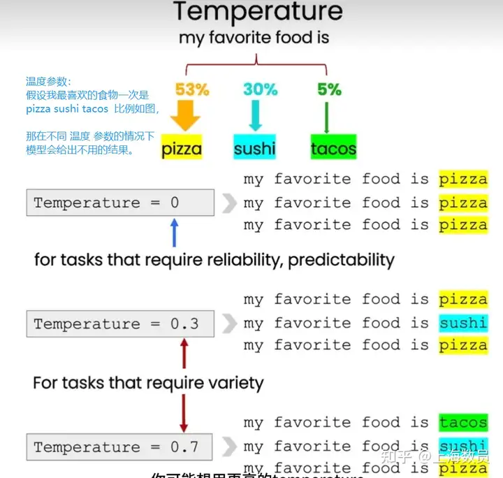
The word selection is based on top_p and top_k, which are used to prevent the generated result from going into the loop The top_k parameter is used to select the top k probability tokens as the next candidate tokens
def top_k_logits(logits, k): ## calculate top_k
    if k == 0:
        # no truncation
        return logits

    def _top_k():
        values, _ = tf.nn.top_k(logits, k=k)
        min_values = values[:, -1, tf.newaxis]
        return tf.where(
            logits < min_values,
            tf.ones_like(logits, dtype=logits.dtype) * -1e10,
            logits,
        )
    return tf.cond(
       tf.equal(k, 0),
       lambda: logits,
       lambda: _top_k(),
    )
The top_p method is used to select the first few tokens in the candidate tokens whose probability accumulation reaches the p threshold as the next candidate tokens
ef top_p_logits(logits, p):  ### Calculate top_p. If it is equal to 1, it is equivalent to no calculation
    with tf.variable_scope('top_p_logits'):
        logits_sort = tf.sort(logits, direction='DESCENDING')
        probs_sort = tf.nn.softmax(logits_sort)
        probs_sums = tf.cumsum(probs_sort, axis=1, exclusive=True)
        logits_masked = tf.where(probs_sums < p, logits_sort, tf.ones_like(logits_sort)*1000) # [batchsize, vocab]
        min_logits = tf.reduce_min(logits_masked, axis=1, keepdims=True) # [batchsize, 1] # Extract slices from sorted_logits in the format of indices
        return tf.where(  # If condition=True, the X value is returned, and if False, the Y value is returned
            logits < min_logits,
            tf.ones_like(logits, dtype=logits.dtype) * -1e10,
            logits,
        )
With the output parameters out of the way, let's look at the gpt2-finetuning example output process:
def sample_sequence(*, hparams, length, start_token=None, batch_size=None, context=None, temperature=1, top_k=0, top_p=0.0):
    if start_token is None:
        assert context is not None, 'Specify exactly one of start_token and context!'
    else:
        assert context is None, 'Specify exactly one of start_token and context!'
        context = tf.fill([batch_size, 1], start_token)   #value=1 fill() Start with token

    def step(hparams, tokens, past=None):
        lm_output = model.model(hparams=hparams, X=tokens, past=past, reuse=tf.AUTO_REUSE)

        logits = lm_output['logits'][:, :, :hparams.n_vocab]
        presents = lm_output['present']
        presents.set_shape(model.past_shape(hparams=hparams, batch_size=batch_size))
        return {
            'logits': logits,
            'presents': presents,
        }

    with tf.name_scope('sample_sequence'):
        def body(past, prev, output):
            next_outputs = step(hparams, prev, past=past)    # shape=(1, ?, 50257)
            logits = next_outputs['logits'][:, -1, :]  / tf.to_float(temperature)    ## As long as the last output value (probability vector of possible values)
            if top_p > 0.0:
                logits = top_p_logits(logits, p=top_p)
            else:
                logits = top_k_logits(logits, k=top_k)   ## [0,0,0.2,0,1,] probability
            samples = tf.multinomial(logits, num_samples=1, output_dtype=tf.int32)  #logits is a two-dimensional tensor, and num_samples refers to the number of samples. It's easy to understand that when we generate the logits for each time, the output dimension should be of the form [batch_size, vocab_size], which represents the probability of each word in the dictionary for each batch at that time. multinomial() will sample from this probability distribution and return the id of the second dimension of the logits, which is the dictionary id we need.

            return [
                next_outputs['presents'] if past is None else tf.concat([past, next_outputs['presents']], axis=-2),  #present is the [k,v] for each layer.
                samples,
                tf.concat([output, samples], axis=1)
            ]

        past, prev, output = body(None, context, context)

        def cond(*args):
            return True

        _, _, tokens = tf.while_loop(     #The loop loop_vars is both the output value and the input for the next iteration of the loop
            cond=cond, body=body,
            maximum_iterations=length - 1,
            loop_vars=[
                past,
                prev,
                output
            ],
            shape_invariants=[
                tf.TensorShape(model.past_shape(hparams=hparams, batch_size=batch_size)),
                tf.TensorShape([batch_size, None]),
                tf.TensorShape([batch_size, None]),
            ],
            back_prop=False,
        )

        return tokens
1.5 Finding the Words to Say: Hidden State Visualizations for Language Models
The following describes how we will visualize the hidden layer and find the logic of gpt picking tokens
This section is a summary of the articleJay Alammar-Finding the Words to Say: Hidden State Visualizations for Language Models
Code:https://colab.research.google.com/github/jalammar/ecco/blob/main/
Visualization: As the model generates sentences, list each output word in the order of its score in that layer, with a color representing its rank. 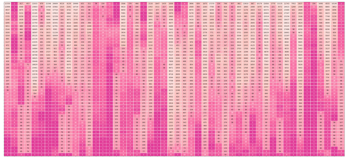
1.5.1 Scores after each layer
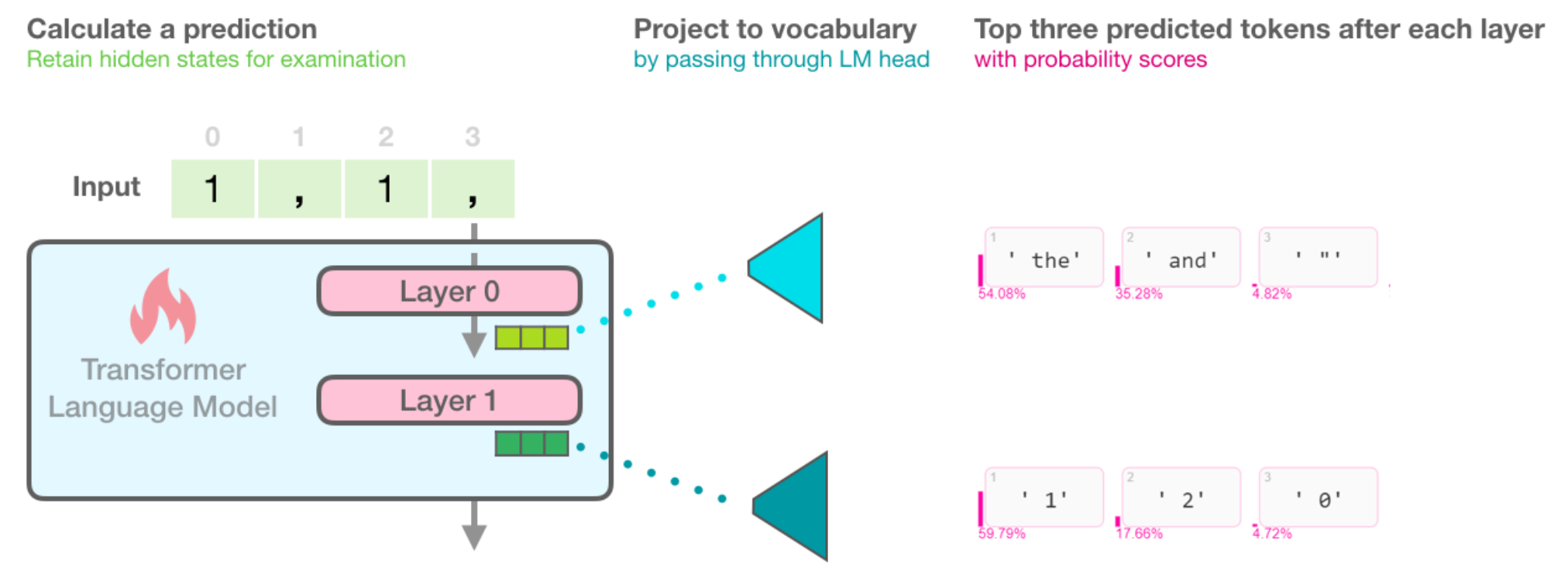
The figure below illustrates how the Transfromer-based language model operates between layers to obtain the hidden states and how the final tokens are mapped into this table and a token score is given to other possible tokens. For example, when given "1,1,", the model knows the next word to be "1" 59% of the time and "2" 18% of the time (maybe we're counting positively). 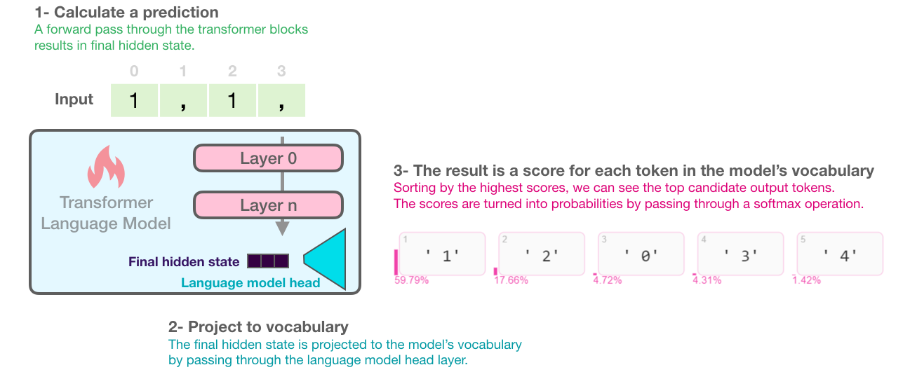
The open-source code used in the paper, Ecco, provides the token with the highest model score along with other candidate tokens and their probability scores.
# Generate one token to complete this input string
output = lm.generate(" 1, 1, 1,", generate=1)

# Visualize
output.layer_predictions(position=6, layer=5)
In addition, except for the probability score representation for the final result layer, the output of each layer is represented by probability scores
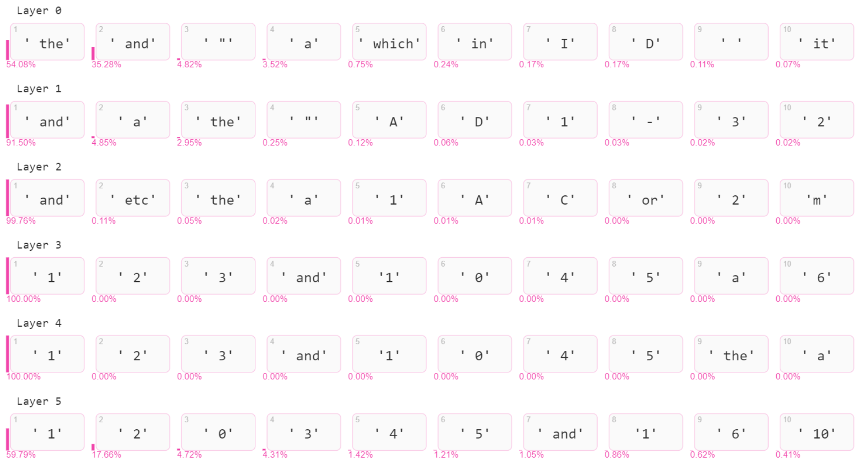
Combining the output probability score representations of each layer above, we can obtain a token probability score matrix as follows: (Each row gets the output word by projecting the hidden state onto the vocabulary, and softmaxes its logits score to get the probability score. In this example, there are no predicted numbers in the first ten digits of layer 0, and "1" in layer 1 is only 0.03 probability, but "1" in layer 1 is 100% probability distribution. The final layer diverts the probabilities using the parameters mentioned in the previous section, resulting in a probability score of 59%.)
1.5.2 Evolution of the selected token
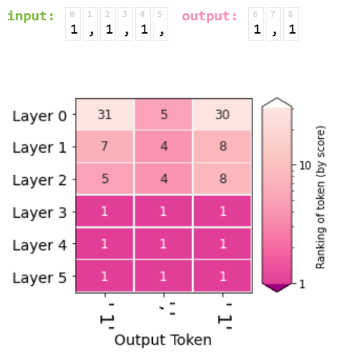
Another visualization is to summarize the rank of the final result (that is, the "1") at each level as follows: 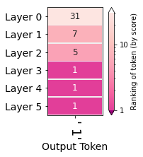 You can see that "1" is ranked 31st in layer 0, and has been ranked first since layer 3
Let's extend the second method to represent the cumulative state of the subsequent outputs, for example, the input "1,1,1," and let's now represent the rank of the output "1,1" in each layer as shown:
Here is a demonstration of the usual prompt sentence, When we type:
"The country of the European Union are : \n "
"1 . Austria \n"
"2 . Belgium \n"
"3 . Bulgaria \n"
"4."
By visualizing the hidden layers, we can see how each layer selects words and their impact on the final output:  We can see that for newline characters and periods, the model has already flagged them and has not objected to them since. After the ninth layer, the model correctly predicts the numbers "5" and "6" incrementing. It is worth noting that the model incorrectly added chile to the list of EU countries, but it was not the model itself that was wrong, as "chile" was 43rd in the list of model predictions. The model output should be modified by checking the sampling parameters we mentioned in the previous section. (Also, in addition to predicting the countries, the model correctly alphabetical the countries.)
1.5.3 Evolution of the selected token
In addition to the probabilistic ranking evolution of the output token, we also want to be able to get the probabilistic evolution of other tokens. For example, for the model to analyze simple, complex and main clause objects, we can input:
"The only acceptable answers are 1) is 2) are"
"The keys to the cabinet __"
To see if the model knows whether we're mainly talking about keys or cabinet. After determining the subject, we decide whether to use "is" or "are". In the figure below, we can see how the model ranks the probabilities for is or are by layer 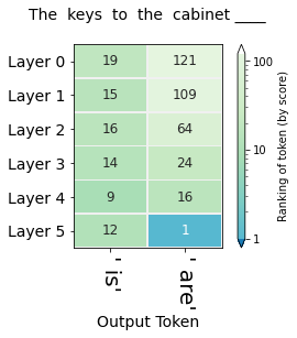
Similarly, we could change the title to:
"The key to the cabinets__"
The probability ranking map of each layer is obtained: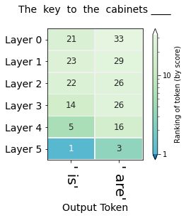
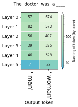
In this way, we can explore how the model can generate biases, such as gender expectations for different occupations 